Preamble

This post is part of an effort to document the cohort-component method in a comprehensive und practical way.
It is work in progress, and put online hoping it is useful. Suggestions and corrections welcome!

The text was taken from unpublished write-ups in MS Word (247 formulas in MathType) and turned semi-automatically (using pandoc) into a html document. Mathematical equations and symbols are originally created in MathType for Word, then converted into PlainTeX.
There are still many problems (charts, tables, other references than ToC [eqn. references, ..]) waiting for solutions.

1 Introduction
2 Synopsis: Cohort-component projection for open populations
3 Closed population
- 3.1 Forward Projection
- 3.2 Calculation of cohort deaths
4 Open population
5 Indicators and symbols
6 Bibliography

1 Introduction

The following text summarizes basic mathematical approaches to population projections using the cohort-component method, including the calculation of deaths and their subsequent transformation into deaths by age. Most of these formulas are well established, but rarely comprehensively documented and presented together with their derivation. Thus, by pulling together different sources and using different approaches, the text tries to provide a systematic description of the underlying algebra and the relationships between the demographic components.

This document is based on employing the period life table as the basis for developing the mathematics of population projections, including the calculation of associated deaths. It is helpful to recall that the L_x column of the life table represents the person-years lived of a life table population and therefore represents a (stationary) population. Consequently, using the L_x column of the life table and associated statistics (like the survivor proportion), it is possible to develop the cohort component projection method. There are other approaches to formulate the cohort-component method, but they are not covered here¹.

This document and its annexes also includes an extension to the usual calculation of deaths in a cohort component projection, namely for the explicit calculation of deaths to the last closed age group. This extension was prompted by the availability of revised model life tables extended to a highest age of 130 years (see UNPD 2015). Some extra attention is paid to the adequate exposed-to-risk for the early years of life, for the time from birth to age one and age five.

Another rarely covered element of calculating cohort component projection is the calculation of deaths by age and sex. Deaths in a cohort-component framework are associated with the survival of cohorts of people of the same years of birth, they are, in Lexis’s terms, period-cohort events. Because deaths produced by statistical agencies are normally formatted according to a period-age observation plan, the deaths calculated in a cohort component projection need to be transformed to that format. The transformation of cohort deaths into deaths by age and sex can be achieved by applying cohort-separation factors obtained from a life table, as shown in general terms in Annex II.

There are topics not yet covered, among them methods for reverse-projection and the methodology of multiregional projections.

2 Synopsis: Cohort-component projection for open populations

2.1 Forward projection

For this approach to calculate forward projection for populations open to migration, the (net) migration by age need to be re-arranged into a cohort format:

${}_n^cM_x^{t,t + n} = {1 \over 2}{}_nM_x^{t,t + n} + {1 \over 2}{}_nM_{x + n}^{t,t + n}$

2.1.1 Births

Births are calculated by multiplying age-specific fertility rates to (female) population at risk during the interval, including the contribution made by migrant women in the reproductive age. Since net migration is predominantly being used in national projections, migration figures can be positive (excess of immigrant) or negative (excess of emigrants). Consequently, the contribution of migrants in following formula might be positive or. Negative net migration produces negative births, that is births that would have occurred in the country had the woman not emigrated. Since the outmigration has not been considered in the calculation of the births attributable to the female population present at the beginning of the period, those “lost” births need to be subtracted.

${}_nB_x^{t,t + n} = n*{}_nF_x^{t,t + n}*\left[ {{1 \over 2}\left( {{}_nP_x^t + {}_nP_{x - n}^t*{}_nS_{x - n}^{t,t + 1}} \right) + {}_n^cM_x^{t,t + n}{1 \over 2}\left( {1 + {}_nS_x^{t,t + n}} \right)} \right]$

2.1.2 Survival of births

Births are forward survived by using the following formula. Note that migrants born during the interval are factored-in by applying two thirds of the mortality in the interval.

${}_nP_0^{t + n} = {B^{t,t + n}}*{{{}_nL_0^{t,t + n}} \over {n*{l_0}}} + {1 \over 2}*M_0^{t,t + n}*{1 \over 3}*\left( {1 + 2*{{{}_nL_0^{t,t + n}} \over {n*{l_0}}}} \right)$

2.1.3 Projecting closed age groups

The forward projection is then done using the following formula for ages $x{\rm{ }} = {\rm{ }}0,{\rm{ }}n,{\rm{ }}2n,{\rm{ }} \ldots ,{\rm{ }}z - 2n$ ;

${}_nP_{x + n}^{t + n} = \left[ {{}_nP_x^t*{}_nS_x^{t,t + n}} \right] + {}_n^cM_x^{t,t + n}*{1 \over 2}\left( {1 + {}_nS_x^{t,t + n}} \right)$

2.1.4 Projecting the last, open-ended age group, standard age format

The open-ended age group at time t+n is composed of the survivors of the last closed age group at time t plus the survivors of the open-ended age group at time t. Population projections are usually prepared with life tables having the same ultimate age group as the population to be projected. In such a case, the last closed age group, and the open-ended age group of the population at time t need be combined and projected together.

Case: $\omega = z$
First, the last two age groups of the population at time t are aggregated into a new last, open-ended age group starting at age $z - n = \omega - n$ :

${}_\infty P_{z - n}^t = \left( {{}_nP_{z - n}^t + {}_\infty P_z^t} \right)$

For the corresponding migration in period-cohort format, half the migration in age group z-n und all the last, open-ended age group, is to be combined

${}_\infty ^cM_{z - n}^{t + n} = {1 \over 2}{}_nM_{z - n}^{t.t + n} + {}_\infty M_z^{t,t + n}$

The survivor ratio for the last age group is taken from the life table statistic ${T_x}$ _, e.g. “persons years lived above age x”

${}_\infty S_{z - n}^{t,t} = {{T_z^{t,t + n}} \over {T_{z - n}^{t,t + n}}}$

After these preparatory steps, the forward projection can be performed

${}_\infty P_z^{t + n} = \left( {{}_\infty P_{z - n}^t} \right)*{{T_z^{t,t + n}} \over {T_{z - n}^{t,t + n}}} + {}_\infty ^cM_{z - n}^{t.t + n}*{1 \over 2}*\left( {1 + {{T_z^{t,t + n}} \over {T_{z - n}^{t,t + n}}}} \right)$

and simplified

${}_\infty P_z^{t + n} = \left( {{}_\infty P_{z - n}^t} \right)*{}_\infty S_{z - n}^{t,t} + {}_\infty ^cM_{z - n}^{t.t + n}*{1 \over 2}*\left( {1 + {}_\infty S_{z - n}^{t,t}} \right)$

This formula assumes that population age structure is stationary beginning at age z-n. Another implication of this formula is that deaths by age group can only be calculated for the last two age groups.

An approach that avoids these implications is presented next.

2.1.5 Projecting the last, open-ended age group, extended age format

Case $\left( {\omega \ge z + n} \right)$
In case the underlying life table has more age groups than the population, calculations can be done in more detail by separating the last closed age group from the last open-ended age group. First, migrants are re-arranged into two cohort age groups. Note that splitting the last age group in half to estimate cohort events is a rough approximation, especially if there is still sizable migration happening in that age group.

$\eqalign{ & {}_n^cM_{z - n}^{t,t + n} = {1 \over 2}{}_nM_{z - n}^{t,t + n} + {1 \over 2}{}_\infty M_z^{t,t + n} \cr & {}_\infty ^cM_z^{t,t + n} = {1 \over 2}{}_\infty M_z^{t,t + n} \cr}$

With the cohort migration in place, we can project according to the following formula:

$\matrix{ {{}_\infty P_z^{t + n}} \hfill & = \hfill & {{}_nP_{z - n}^t*{}_nS_{z - n}^{t,t + n} + {}_\infty P_z^t*\left( {{{T_{z + n}^{t,t + n}} \over {T_z^{t,t + n}}}} \right)} \hfill \cr {} \hfill & {} \hfill & { + {}_n^cM_{z - n}^{t + n}*{1 \over 2}*\left( {1 + S_{z - n}^{t,t + n}} \right)} \hfill \cr {} \hfill & {} \hfill & { + {}_\infty ^cM_z^{t + n}*{1 \over 2}*\left( {1 + {{T_{z + n}^{t,t + n}} \over {T_z^{t,t + n}}}} \right)} \hfill \cr }$

This formula assumes that the population age structure is stationary beginning at age z.

Note that Hill (1990, p. 50) suggest splitting the migrants differently. (to be added)

2.2 Calculation of deaths

Deaths calculated in the context of a cohort-component model are deaths according to a period-cohort observation plan, or cohort deaths for short.

2.2.1 Births

Following a suggestion made by Pollard, the migrants born during the period are exposed to two-thirds of the overall mortality occurring between births and the end of the projection period. Note that these deaths are occurring in a lower Lexis triangle (denoted with left superscript l).

${}_n^lD_0^{t,t + n} = {B^{t,t + n}}*\left( {1 - {{{}_nL_0^{t,t + n}} \over {n*{l_0}}}} \right) + {1 \over 2}*{}_nM_0^{t,t + n}*{2 \over 3}*\left( {1 - {{{}_nL_0^{t,t + n}} \over {n*{l_0}}}} \right)$

2.2.2 Closed age groups

The total number of deaths in a closed age group for ages $x{\rm{ }} = {\rm{ }}0,{\rm{ }}n,{\rm{ }}2n,{\rm{ }} \ldots ,{\rm{ }}z - n$ is calculated according to the following formula:

$\matrix{ {{}_n^cD_x^{t,t + n}} \hfill & = \hfill & {{}_nP_x^t*\left( {1 - {}_nS_x^{t,t + n}} \right)} \hfill \cr {} \hfill & {} \hfill & { + {}_n^cM_x^{t,t + n}*{1 \over 2}\left( {1 - {}_nS_x^{t,t + n}} \right)} \hfill \cr }$

Recall the rearrangement of migrants by age into a cohort format according to the formulas:

${}_n^cM_x^{t,t + n} = {1 \over 2}{}_nM_x^{t,t + n} + {1 \over 2}{}_nM_{x + n}^{t,t + n}$

Note that for the penultimate age group, it is assumed that the cohort migrants are composed of half the migrants in age group z-n and half of the last, open- ended age group z.

${}_\infty ^cM_{z - n}^{t,t + n} = {1 \over 2}{}_nM_{z - n}^{t,t + n} + {1 \over 2}{}_\infty M_z^{t,t + n}$

2.2.3 Last, open-ended age group

We distinguish two different cases.

Case: $\omega \ge z + n$
Deaths occurring to the last open-ended age group are calculated as follows.

${}_\infty ^cM_z^{t,t + n} = {1 \over 2}{}_\infty M_z^{t,t + n}$

$\matrix{ {{}_\infty ^cD_z^{t,t + n}} \hfill & = \hfill & {{}_\infty P_z^t*\left( {1 - {{T_{z + n}^{t,t + n}} \over {T_z^{t,t + n}}}} \right)} \hfill \cr {} \hfill & {} \hfill & { + {}_\infty ^cM_z^{t,t + n}*{1 \over 2}\left( {1 - {{T_{z + n}^{t,t + n}} \over {T_z^{t,t + n}}}} \right)} \hfill \cr }$

2.3 Transformation of cohort deaths into death by age

Deaths calculated in a cohort-component framework are cohort deaths, or, in Lexis terms, deaths in a Period-Cohort format [P-C]. This segment shows the transformation of cohort deaths into deaths by age (Period-Age format, [P-A]). For details, see Annex II.

2.3.1 First age group

The first age group in [P-A] format consists of the lower triangle deaths that are associated with the survival of births to the end of the period, plus the upper triangle of the first full cohort age group.

${}_nD_0^{t,t + n} = {}_n^lD_0^{t,t + n} + {}_n^uD_0^{t,t + n}$

The lower triangle has already been calculated (see 2.2.1.). The upper triangle can be calculated using the corresponding cohort separation factor (see 6.1).

${}_n^uD_0^{t,t + n} = {}_n^cD_0^{t,t + n}*{}^c{\rm{f}}_0^{t,t + n}$

The total number of deaths in the first age group [x=0, n] can then be calculated as:

${}_nD_0^{t,t + n} = {}_n^lD_0^{t,t + n} + {}_n^cD_0^{t,t + n}*{}^c{\rm{f}}_0^{t,t + n}$

2.3.2 Other closed age groups

The other closed age groups in Period-Age format are calculated by applying appropriate cohort-separation factors and rearranging the resulting Lexis triangles.

$\matrix{ {{}_nD_x^{t,t + n}} \hfill & = \hfill & {{}_n^lD_x^{t,t + n} + {}_n^uD_x^{t,t + n}} \hfill \cr {} \hfill & = \hfill & {{}_n^cD_{x - n}^{t,t + n}*\left( {1 - {}^c{\rm{f}}_{x - n}^{t,t + n}} \right)} \hfill \cr {} \hfill & {} \hfill & { + {}_n^cD_x^{t,t + n}*{}^c{\rm{f}}_x^{t,t + n}} \hfill \cr }$

$x{\rm{ }} = {\rm{ }}n,{\rm{ }}2n,{\rm{ }} \ldots ,{\rm{ }}z - n$ .

2.3.3 Last, open-ended age group

If the underlying life table provides more age groups than the population, than the deaths by age starting at age z-n can be calculated by the above formula. The last open-ended age group beginning at age z is then the sum of the cohort death associated with the last age plus a fraction from the last closed age group.

Case $\left( {\omega \ge z + n} \right)$
$\matrix{ {{}_\infty D_z^{t,t + n}} \hfill & = \hfill & {{}_n^cD_{z - n}^{t,t + n}*{}^c{\rm{f}}_{z - n}^{t,t + n}} \hfill \cr {} \hfill & {} \hfill & { + {}_\infty ^cD_z^{t,t + n}} \hfill \cr }$

2.3.4 Approximation I

If projections are calculated in single-year-of-age format, then cohort separation factors may be set to 0.5 as a reasonable first approximation. Since the non-linear probability of dying during the first year of life is already reasonably well accounted for in the first lower Lexis triangle, such a shortcut seems appropriate.

${}_n^PD_0^{t,t + n} = {}_n^lD_0^{t,t + n} + {1 \over 2}{}_n^cD_0^{t,t + n}$

${}_n^PD_x^{t,t + n} = {1 \over 2}*{}_n^cD_{x - n}^{t,t + n} + {1 \over 2}{}_n^cD_x^{t,t + n}$

${}_\infty ^PD_z^{t,t + n} = {1 \over 2}*{}_n^cD_{z - n}^{t,t + n} + {}_\infty ^cD_z^{t,t + n}$

2.3.5 Approximation II

The simple approximation under 2.3.4. can be improved by iteratively refining the (empirical) cohort separation factors. This is especially useful for the first and last age groups. It is advisable to use such refinement when the age groups are larger than one year.

Set the cohort separation factor fc to halve the age interval
Calculate the death according to the period-age observation plan by using the cohort-separation factors.
Calculate life tables statistics m_x, a_x, q_x (or p_x), l_x and L_x. Obtain updated cohort separation factors from the life table statistics.
Repeat with step 2 or stop.

3 Closed population

First, the cohort-component method is developed for population closed to migration. This allows for a streamlined derivation of the basic mathematical relations. Note that the document does not distinguish between male and female populations but assumes a female-dominant population.

3.1 Forward Projection

It is useful to distinguish four different tasks for the projection of a population:

The calculation of births by age of mother
The survival of births to the end of the projection interval
The projection of cohorts already born except the last-open-ended age group (closed age groups),
The projection of the last, open-ended age group.

For the symbols employed throughout the text, see Annex I.

3.1.1 Births

The births during the projection period are the basis for calculation the first age group of the projected population. Births by age of mother are calculated by multiplying age-specific fertility rates with exposed to risk female population

${}_nB_x^{t,t + n} = n*{}_nF_x^{t,t + n}*{1 \over 2}\left( {{}_nP_x^t + {}_nP_x^{t + n}} \right)$

Note that population exposed to the risk of childbearing belongs to the same age group but at different points in time and is therefore not a cohort format. Using the projection formulas for a closed population, births by age of mother can be calculated without first executing the projection:

${}_nB_x^{t,t + n} = n*{}_nF_x^{t,t + n}*{1 \over 2}\left( {{}_nP_x^t + {}_nP_{x - n}^t*{}_nS_{x - n}^{t,t + n}} \right)$

Total births are then obtained by summing the births by age of mother for all age groups of reproductive age.

${B^{t,t + n}} = \sum\limits_{x = 15}^{50 - n} {{}_nB_x^{t,t + n}}$

3.1.2 Survival of births

The births born during period [t, t+n] need to be forward survived to the end of the projection period. The survivor ratio for forward surviving the births to the end of the projection period is the proportion of the radix of the life table l₀ (the births) to the person-years-lived for the first age group of the life table _nL₀.

${}_nP_0^{t + n} = {B^{t,t + n}}*{{{}_nL_0^{t,t + n}} \over {n*{l_0}}}$

3.1.3 Projecting closed age groups

The population in age group [x, x+n] at time t is forward survived/projected to time t+n and age group [x+n, x+2n] using ratios of life table person-year lived (_nL_x) or survivor ratios (_nS_x) as follows ( $x = 0,n,2n,...,z - 2n$ )

${}_nS_x^{t,t + n} = {{{}_nL_{x + n}^{t,t + n}} \over {{}_nL_x^{t,t + n}}}$

${}_nP_{x + n}^{t + n} = {}_nP_x^t*{}_nS_x^{t,t + n}$

3.1.4 Projecting the last, open-ended age group, standard age format

Case: $\omega = z$
$\matrix{ {{}_\infty P_z^{t + n}} \hfill & = \hfill & {\left( {{}_nP_{z - n}^t + {}_\infty P_z^t} \right)*{{T_z^{t,t + n}} \over {T_{z - n}^{t,t + n}}}} \hfill \cr {} \hfill & = \hfill & {\left( {{}_nP_{z - n}^t + {}_\infty P_z^t} \right)*{{\sum\limits_{x = z}^\omega {L_x^{t,t + n}} } \over {\sum\limits_{x = z - n}^\omega {L_x^{t,t + n}} }}} \hfill \cr }$

This formula assumes that population age structure is stationary beginning at age z-n. Another implication of this formula is that deaths by age group can only be calculated for the last two age groups combined – the deaths of the last closed age group [z-n, n] are not separately available.

An approach that avoids these implications is presented next.

3.1.5 Projecting the last, open-ended age group, extended age format

If the underlying life table has at least one more age groups than the population to be projected, the last closed age group and the open-ended age group can be projected separately. This limits the assumption of stationarity to the last, open-ended age group and, at the same time, allows for the calculation of deaths for all age groups, including the last closed age group (shown later).

Case: $\omega \ge z + n$
Recall also that the last open-ended age group at time t+n is composed of the survivors of the last closed age group plus the survivors of the open-ended age group. The projected population at the end of the projection interval is then

${}_\infty P_z^{t + n} = {}_nP_z^{t + n} + {}_\infty P_{z + n}^{t + n}$

The survivors of the last closed age group at time t are then

$\matrix{ {{}_nP_z^{t + n}} \hfill & = \hfill & {{}_nP_{z - n}^t*{}_nS_x^{t,t + n}} \hfill \cr {} \hfill & = \hfill & {{}_nP_{z - n}^t*{{{}_nL_z^{t,t + n}} \over {{}_nL_{z - n}^{t,t + n}}}} \hfill \cr }$

The survivors of the open-ended age group at time t+n are calculated by using a $T_x^{t,t + n}$ where x = z + n, which is beyond the last age of the population under consideration.

${}_\infty P_{z + n}^{t + n} = {}_\infty P_z^t*{{T_{z + n}^{t,t + n}} \over {T_z^{t,t + n}}}$

Combining the formulas gives an expression for the last open-ended age group:

$\matrix{ {{}_\infty P_z^{t + n}} \hfill & = \hfill & {{}_nP_{z - n}^t*{}_nS_x^{t,t + n} + {}_\infty P_z^t*{{T_{z + n}^{t,t + n}} \over {T_z^{t,t + n}}}} \hfill \cr {} \hfill & = \hfill & {{}_nP_{z - n}^t*{{{}_nL_z^{t,t + n}} \over {{}_nL_{z - n}^{t,t + n}}} + {}_\infty P_z^t*{{T_{z + n}^{t,t + n}} \over {T_z^{t,t + n}}}} \hfill \cr }$

3.2 Calculation of cohort deaths

The cohort component method operates along cohort lines: The population in age group x to x+n at time t is moved forward to time t+n and age group x+n to x+2n. The deaths associated with such an approach are here called cohort deaths and labeled ^cD_x. The calculation of cohort deaths (according to a period-cohort observation plan) in a close population are shown next.

Implementing the calculation of deaths in a cohort-component framework is complicated as the results by age are (1.) according to a period-cohort observation plan, and (2.) is generating a Lexis triangle for its first element.

3.2.1 Births

We start with deaths occurring to births until the end of the projection interval. These deaths are occurring in a lower Lexis triangle, denoted with l.

. $\matrix{ {{}_n^lD_0^{t,t + n}} \hfill & = \hfill & {{B^{t,t + n}}*\left( {1 - {{{}_nL_0^{t,t + n}} \over {n*{l_0}}}} \right)} \hfill \cr {} \hfill & = \hfill & {{B^{t,t + n}}*\left( {{{n*{l_0} - {}_nL_0^{t,t + n}} \over {n*{l_0}}}} \right)} \hfill \cr }$ .

Note that the numerator $n*{l_0} - {}_n{L_0}$ is the equivalent of the deaths in the first, lower Lexis triangle (births during the interval minus survivor at the end of the interval).

3.2.2 Closed age groups

Next, the cohort deaths for cohorts already born are calculated, except for the last, open-ended age group. The left superscript c labels the deaths as cohort deaths.

$\matrix{ {{}_n^cD_x^{t,t + n}} \hfill & = \hfill & {{}_nP_x^t*\left( {1 - {}_nS_x^{t,t + n}} \right)} \hfill \cr {} \hfill & = \hfill & {{}_nP_x^t*\left( {1 - {{{}_nL_{x + n}^{t,t + n}} \over {{}_nL_x^{t,t + n}}}} \right)} \hfill \cr {} \hfill & = \hfill & {{}_nP_x^t*\left( {{{{}_nL_x^{t,t + n} - {}_nL_{x + n}^{t,t + n}} \over {{}_nL_x^{t,t + n}}}} \right)} \hfill \cr }$

Note that the numerator $\left( {{}_nL_x^{t,t + n} - {}_nL_{x + n}^{t,t + n}} \right)$ is the life table equivalent of the cohort deaths that we wish to calculate for the population projection.

Note that the age range applicable for the calculation of closed age groups is different depending on the availability of extended life tables:

3.2.3 Last, open-ended age group, standard age format

If the base population and the underlying life table share the same last age (z=ω), then the following approach for the calculation of the last, open-ended age group must be used.

Case: $\omega = z$
${}_\infty ^cD_{z - n}^{t + n} = \left( {{}_nP_{z - n}^t + {}_\infty P_z^t} \right)*\left( {1 - {{T_z^{t,t + n}} \over {T_{z - n}^{t,t + n}}}} \right)$

Note that in this case the deaths for the last open-ended age group start at z-n.

3.2.4 Last, open-ended age group, extended age format

If a life table with at least one more age group then is available for the population is used, then deaths can be calculated for all age groups, including the last closed population age group.

Case: $\omega \ge z + n$
Deaths occurring to the last open-ended age group are calculated as follows.

${}_\infty ^cD_z^{t,t + n} = {}_\infty P_z^t*\left( {1 - {{T_{z + n}^{t,t + n}} \over {T_z^{t,t + n}}}} \right)$

Note that in the case of extended age formats, the last open-ended age group starts at age z.

4 Open population

The projection of population open to migration follows the same steps as outlined for a closed population. The one difference is to account for the effects of (international) net migration.

Basically, migration could be treated the same way as births or deaths: immigration adds to the population, and emigration reduces the population.

There are several approaches to incorporate migration.

One popular approach, outlined in Preston et al. (2001, 24 pp), is presented below. This approach divides net migration (by cohorts) into two parts, of which half is added to the population at the beginning of the period, and half is added to the end. Such an approach exposes half the migration added to the beginning to the full amount of mortality, and excludes the other half that is added at the end of the period from the risk of dying. By adding half of the migration of the next age group to the population at the end, this approach operates, albeit implicitly, on cohorts. This approach for integrating migration into the cohort-component framework is called “Split migration option” in this document.

The approach is correcting a few errors in the formulas presented in Preston (2001). In addition, it is extended for the calculation of deaths.

Another, but similar, approach is more compact and operates under the assumption that migration enters/leaves the population exactly at mid-period, exposing all the migration to half of the mortality. Note that in this approach, migration needs to be transformed explicitly into cohorts, usually by splitting age groups into halves and then re-arranging them into cohorts. This approach will be called “Mid-period option” throughout this document².

It is important to note that both approaches produce reasonable approximations but rest on a few assumptions. Because the cohort-component method acts on cohorts, the usual migration figures by age group need to be re-arranged into cohort age groups. Both approaches mentioned Splitting age groups by half implies that net migration does not change significantly between two adjacent age groups. Errors incurred by these simplifications are larger in the context of five-year age groups and smaller in single year age groups.

Both approaches are documented separately.

This document contains a minor innovation by following up on a suggestion by Preston et al. (2001) to project the last, open-ended age group in a cohort-projection by separating the projection of the two age groups involved (the last closed and the open-ended age group) separately. Such an approach has two advantages:

It relaxes the implicit assumption about the stationarity of the last population age groups from applying to the last two age groups to only the last (open-ended) age group.
It allows calculating deaths for the last closed age group and for the last, open-ended age group separately.

Such an approach requires having an underlying life table with at least one more age group than the population to be projected. As Preston et al. (2001) did not apply this approach in their book, this document is probably the first documenting it comprehensively.

4.1 Forward projection, split migration option

4.1.1 Births

First, births need to be calculated by also factoring in the effects of net-migration, that’s the impact of an increasing or decreasing population exposed to the risk of giving birth³.

It is helpful to develop the formulas separately for births born by the (female) population present at the beginning of the projection interval and those born to (female) migrants that entered during the projection interval. The births born by mothers present at the beginning of the interval (initial-at-risk) are calculated using the formula for a closed population.

${}_nBp_x^{t,t + n} = n*{}_nF_x^{t,t + n}*{1 \over 2}\left( {{}_nP_x^t + {}_nP_x^{t + n}} \right)$

Note that for an open population, the (female) population at time t+n at age x would already include net migration occurring during period [t, t+n]. By forward surviving the population at age x-n at time t to time t+n and age group x using survivor ratios, we get the person –years lived for those present at the beginning of the projection interval⁴:

${}_nBp_x^{t,t + n} = n*{}_nF_x^{t,t + n}*{1 \over 2}\left( {{}_nP_x^t + {}_nP_{x - n}^t*{}_nS_{x - n}^{t,t + 1}} \right)$

The births by age of migrating mother (in or out) are calculated similarly, by replacing the population at risk at age x with half the migrants at risk during period [t, t+n] at age x⁵:

${}_nBm_x^{t,t + n} = n*{}_nF_x^{t,t + n}*{1 \over 2}\left( {{1 \over 2}{}_nM_x^{t,t + n} + {1 \over 2}{}_nM_{x - n}^{t,t + n}*{}_nS_{x - n}^{t,t + n}} \right)$

Combining the two components results in the births by age of mother during period [t, t+n] for a population open to migration:

${}_nB_x^{t,t + n} = {}_nBp_x^{t,t + n} + {}_nBm_x^{t,t + n}$

And written explicitly:

$\matrix{ {{}_nB_x^{t,t + n}} \hfill & = \hfill & {n*{}_nF_x^{t,t + n}*{1 \over 2}\left( {{}_nP_x^t + {}_nP_{x - n}^t*{}_nS_{x - n}^{t,t + 1}} \right)} \hfill \cr {} \hfill & {} \hfill & { + n*{}_nF_x^{t,t + n}*{1 \over 2}\left( {{1 \over 2}{}_nM_{x - n}^{t,t + n}*{}_nS_{x - n}^{t,t + n} + {1 \over 2}{}_nM_x^{t,t + n}} \right)} \hfill \cr }$

Simplification yields:

${}_nB_x^{t,t + n} = n*{}_nF_x^{t,t + n}*{1 \over 2}\left( {{}_nP_x^t + {1 \over 2}{}_nM_x^{t,t + n} + \left( {{}_nP_{x - n}^t + {1 \over 2}{}_nM_{x - n}^{t,t + n}} \right){}_nS_{x - n}^{t,t + 1}} \right)$

4.1.2 Survival of Births

After the births by age of mother that include the effects of net-migration have been calculated, total births are obtained by adding the births by age group. Note that for surviving births thus obtained to the end of the projection period, another contribution of net-migration still needs to be added. Remember that the births calculated above do not include those newborn migrants that were born during the projection period [t, t+n] by migrants outside the country. They are part of the migrants at age 0 to n.

There are three approaches to deal with this (rather small) component⁶:

Preston et al. suggested adding half the migrants aged 0 at the end of the interval. ${}_nP_0^{t + n} = {B^{t,t + n}}*{{{}_nL_0^{t,t + n}} \over {n*{l_0}}} + {1 \over 2}*{}_nM_0^{t,t + n}$ This is problematic as the migration quantities added at the end are by definition not subject to mortality.
A more accurate solution would be to follow an approach that assumes the migrants that were born during the period are entering/leaving the country at mid period and age aged n/2 years⁷. ${}_nP_0^{t + n} = {B^{t,t + n}}*{{{}_nL_0^{t,t + n}} \over {n*{l_0}}} + {1 \over 2}*M_0^{t,t + n}*{1 \over 2}*\left( {1 + {{{}_nL_0^{t,t + n}} \over {n*{l_0}}}} \right)$ However, this would ignore the uneven distribution of deaths in this age group. It is also likely that children (with their parents) usually do not migrate immediately after births.
Pollard at el. (1974, p. 122) suggest applying two thirds of the survival to those migrants, e.g. two thirds of the mortality in the interval instead of one half. ${}_nP_0^{t + n} = {B^{t,t + n}}*{{{}_nL_0^{t,t + n}} \over {n*{l_0}}} + {1 \over 2}*M_0^{t,t + n}*{1 \over 3}*\left( {1 + 2*{{{}_nL_0^{t,t + n}} \over {n*{l_0}}}} \right)$ Since the overall weight of migrants in the first age group is normally very small when compared to the receiving/sending population, the last two approaches appear to be reasonable. The last option applying two thirds of the overall mortality in the first triangle to half the migrants of that age group appears to be slightly more appropriate, however⁸.

4.1.3 Projecting closed age groups

In the approach suggested by Preston et al., the population at age x at time t is projected forward by applying the survivor ratio at age x for period [t, t+n] to the sum of the population and half the migrants at age x. Half the migration at age x+n is added at the end of the projection interval.

${}_nP_{x + n}^{t + n} = \left[ {\left( {{}_nP_x^t + {1 \over 2}*{}_nM_x^{t,t + n}} \right)*{}_nS_x^{t,t + n}} \right] + {1 \over 2}*{}_nM_{x + n}^{t,t + n}$

Note that combining half the migrants at age x at the beginning of the projection period with half the migrants age x+n to the end of the projection period is following migrants along cohort lines, as required by the cohort-component model.

4.1.4 Projecting the last, open-ended age group, standard age format

The last open-ended age group is composed of the survivors of the last closed age group plus the survivors of the open-ended age group, including migrants. As this version of the inclusion of migrants exposes half of them to the full risk of dying, half of the migrants of the last age group need to be added at the end.

Case $\left( {\omega = z} \right)$
In case the last age for the life table and the population are the same, then the following formula is used:

${}_\infty P_z^{t + n} = \left[ {\left( {{}_nP_{z - n}^t + {}_\infty P_z^t + {1 \over 2}*\left( {{}_nM_{z - n}^{t,t + n} + {}_\infty M_z^{t,t + n}} \right)} \right)*{{T_z^{t,t + n}} \over {T_{z - n}^{t,t + n}}}} \right] + {}_n{1 \over 2}*{}_\infty M_z^{t,t + n}$

Rearranging the formula for the components, one gets:

$\matrix{ {{}_\infty P_z^{t + n}} \hfill & = \hfill & {\left( {{}_nP_{z - n}^t + {}_\infty P_z^t} \right)*{{T_z^{t,t + n}} \over {T_{z - n}^{t,t + n}}}} \hfill \cr {} \hfill & {} \hfill & { + \left( {{1 \over 2}*\left[ {{}_nM_{z - n}^{t,t + n} + {}_\infty M_z^{t,t + n}} \right]} \right)*{{T_z^{t,t + n}} \over {T_{z - n}^{t,t + n}}}} \hfill \cr {} \hfill & {} \hfill & { + {1 \over 2}*{}_\infty M_z^{t,t + n}} \hfill \cr }$

This formula assumes that the population age structure is stationary beginning at age z-n.

4.1.5 Projecting the last, open-ended age group, extended age format

In case the underlying life table has more age groups than the population, the penultimate age group and the last, open-ended age group can be projected separately.

Case $\left( {\omega \ge z + n} \right)$
In this case, the population of the last, open-ended age group is the sum of these two age groups, plus half the migrants of the last open-ended age group at time t+n:

$\matrix{ {{}_\infty P_z^{t + n}} \hfill & = \hfill & {\left( {{}_nP_{z - n}^t + {1 \over 2}*{}_nM_{z - n}^{t,t + n}} \right)*{}_nS_{z - n}^{t,t + n}} \hfill \cr {} \hfill & {} \hfill & { + \left( {{}_\infty P_z^t + {1 \over 2}*{}_\infty M_z^{t,t + n}} \right)*{{T_{z + n}^{t,t + n}} \over {T_z^{t,t + n}}}} \hfill \cr {} \hfill & {} \hfill & { + {1 \over 2}{}_\infty *M_z^{t,t + n}} \hfill \cr }$

If the last, open-ended age group is significantly larger as the preceding closed age group, an equal split into halves may not be justified. Hill suggested to split the last, open-ended age group into ¼ and ¾, respectively (Hill. 1990, p. 50).

$\matrix{ {{}_\infty P_z^{t + n}} \hfill & = \hfill & {\left( {{}_nP_{z - n}^t + {1 \over 2}*{}_nM_{z - n}^{t,t + n}} \right)*{}_nS_{z - n}^{t,t + n}} \hfill \cr {} \hfill & {} \hfill & { + \left( {{}_\infty P_z^t + {1 \over 4}*{}_\infty M_z^{t,t + n}} \right)*{{T_{z + n}^{t,t + n}} \over {T_z^{t,t + n}}}} \hfill \cr {} \hfill & {} \hfill & { + {3 \over 4}{}_\infty *M_z^{t,t + n}} \hfill \cr }$

These formulas assume that the population age structure is stationary beginning at age z.

4.2 Calculation of cohort deaths

4.2.1 Births

Calculation of cohort deaths in an open population are shown next. We start with the deaths occurring to births until the end of the projection interval. These deaths are occurring in a lower Lexis triangle, denoted with superscript l. Note that the effects of net-migration to mothers are already contained in the total number of births. However, deaths experienced by migrants in this age group need to be considered. We start by calculating the deaths attributable to births born in the country during [t, t+n].

${}_n^lD_0^{t,t + n} = {B^{t,t + n}}*\left( {1 - {{{}_nL_0^{t,t + n}} \over {n*{l_0}}}} \right)$

Net-migration contributes twice to the number of deaths occurring to births before reaching the end of the projection interval. First, as mentioned, net-migration adds/subtracts women at risk from the population and thus results in more/less births than would have occurred in the absence of migration. Second, those migrants born during the projection period [t, t+n] either in the country but left before their first birthday or those born outside the country but entered the country before their first birthday also contribute to deaths during the period. However, they are not exactly zero years old, e.g. they enter or leave the country at any age between 0 and n.

As mentioned in 4.1.2. on forward surviving births in an open population, there are three approaches on how to consider migration in that first lexis triangle.

The approach suggested by Preston at al. does not consider the contribution to migrants in the first Lexis triangle. The number of (cohort) deaths is then the same as for the case without migration in that age (note that the contribution of migrant women giving birth is included). ${}_n^lD_0^{t,t + n} = {B^{t,t + n}}*\left( {1 - {{{}_nL_0^{t,t + n}} \over {n*{l_0}}}} \right)$
The second approach assumes that the migrants that were born during the period and entering entering/leaving the country are exposed to the risk of dying half. The contribution of migrants to deaths in the first Lexis triangle is then: ${}_n^lDm_0^{t,t + n} = {1 \over 2}{}_nM_0^{t,t + n}*{1 \over 2}\left( {1 - {{{}_nL_0^{t,t + n}} \over {n*{l_0}}}} \right)$
To calculate the overall deaths occurring in the first Lexis triangle, we combine the formula for births and for migrants and get: ${}_n^lD_0^{t,t + n} = {B^{t,t + n}}*\left( {1 - {{{}_nL_0^{t,t + n}} \over {n*{l_0}}}} \right) + {1 \over 2}*{}_nM_0^{t,t + n}*{1 \over 2}*\left( {1 - {{{}_nL_0^{t,t + n}} \over {n*{l_0}}}} \right)$
A suggestion made by Pollard would expose the migrants to two-thirds of the overall mortality in that Lexis triangle, thereby taking account of the uneven distribution of deaths in this age group ${}_n^lDm_0^{t + n} = {1 \over 2}*M_0^{t,t + n}*{2 \over 3}*\left( {1 - {{{}_nL_0^{t,t + n}} \over {n*{l_0}}}} \right)$ After combining the deaths to migrants and deaths to births, one gets: ${}_n^lD_0^{t,t + n} = {B^{t,t + n}}*\left( {1 - {{{}_nL_0^{t,t + n}} \over {n*{l_0}}}} \right) + {1 \over 2}*{}_nM_0^{t,t + n}*{2 \over 3}*\left( {1 - {{{}_nL_0^{t,t + n}} \over {n*{l_0}}}} \right)$

4.2.2 Closed age groups

Next, the cohort deaths for cohorts already born are calculated, except for the last, open-ended age group. The left superscript c identifies the resulting deaths as cohort deaths. For these age groups, net-migration needs to be incorporated explicitly. Here, we follow the assumption that half the net-migration is subject to the full risk of dying in each closed age group. For calculating the contribution of net-migration to the cohort deaths, use the following formula:

${}_n^cDm_x^{t,t + n} = {1 \over 2}{}_nM_x^{t,t + n}*\left( {1 - {}_nS_x^{t,t + n}} \right)$

The cohort deaths for closed age groups in an open population is then

${}_n^cD_x^{t,t + n} = \left( {{}_nP_x^t + {1 \over 2}{}_nM_x^{t,t + n}} \right)*\left( {1 - {}_nS_x^{t,t + n}} \right)$

4.2.3 Last, open-ended age group

If the base population and the underlying life table share the same last age (z=ω), then the following approach for the calculation of the last, open-ended age group must be used.

Case: $\omega = z$
As in the previous sections, two options are available for the inclusion of migration into the projection formula.

$\matrix{ {{}_\infty ^cD_{z - n}^{t,t + n}} \hfill & = \hfill & {{}_nP_{z - n}^t + {}_\infty P_z^t*\left( {1 - {{T_z^{t,t + n}} \over {T_{z - n}^{t,t + n}}}} \right)} \hfill \cr {} \hfill & {} \hfill & { + \left[ {{1 \over 2}\left( {{}_nM_{z - n}^{t,t + n} + {}_\infty M_z^{t,t + n}} \right)} \right]*\left( {1 - {{T_z^{t,t + n}} \over {T_{z - n}^{t,t + n}}}} \right)} \hfill \cr {} \hfill & {} \hfill & {} \hfill \cr }$

Case: $\omega \ge z + n$
Deaths occurring to the last open-ended age group are calculated as follows.

$\matrix{ {{}_\infty ^cD_z^{t,t + n}} \hfill & = \hfill & {{}_\infty P_z^t*\left( {1 - {{T_{z + n}^{t,t + n}} \over {T_z^{t,t + n}}}} \right)} \hfill \cr {} \hfill & {} \hfill & { + {1 \over 2}{}_\infty M_z^{t,t + n}*\left( {1 - {{T_{z + n}^{t,t + n}} \over {T_z^{t,t + n}}}} \right)} \hfill \cr }$

4.3 Forward projection, mid-period migration option

4.3.1 Births

First, births need to be calculated by also factoring in the effects of net-migration, that’s the impact of an increasing or decreasing population exposed to the risk of giving birth.

It is helpful to develop the formulas separately for births born by the (female) population present at the beginning of the projection interval and those born to (female) migrants that entered during the projection interval. The births born by mothers present at the beginning of the interval are calculated using the formula for a closed population.

${}_nBp_x^{t,t + n} = n*{}_nF_x^{t,t + n}*{1 \over 2}\left( {{}_nP_x^t + {}_nP_x^{t + n}} \right)$

${}_nBp_x^{t,t + n} = n*{}_nF_x^{t,t + n}*{1 \over 2}\left( {{}_nP_x^t + {}_nP_{x - n}^t*{}_nS_{x - n}^{t,t + 1}} \right)$

The births by age of mother born by female migrants are calculated similarly. By combining two age groups of migrants to form a cohort age group and exposing the cohort migrants to the survivor ratio that amounts to half the mortality we arrive at a more compact formula. First the migrants by age are re-arranged to form cohorts:

${}_n^cM_x^{t,t + n} = {1 \over 2}{}_nM_x^{t,t + n} + {1 \over 2}{}_nM_{x + n}^{t,t + n}$

Births to migrants by age of mother are calculated by exposing the age-specific fertility rates to person years lived by the migrants

${}_nBm_x^{t,t + n} = n*{}_nF_x^{t,t + n}*{}_n^cM_x^{t,t + n}*{1 \over 2}*\left( {1 + {}_nS_x^{t,t + n}} \right)$

Now the two sets of events – births by (female) population present at the beginning of the projection interval [t, t+n] and births born by migrating (female) population) – can be combined:

$\matrix{ {{}_nB_x^{t,t + n}} \hfill & = \hfill & {n*{}_nF_x^{t,t + n}*{1 \over 2}\left( {{}_nP_x^t + {}_nP_{x - n}^t*{}_nS_{x - n}^{t,t + 1}} \right)} \hfill \cr {} \hfill & {} \hfill & { + n*{}_nF_x^{t,t + n}*{}_n^cM_x^{t,t + n}*{1 \over 2}\left( {1 + {}_nS_x^{t,t + n}} \right)} \hfill \cr }$

After further simplification, we get

4.3.2 Survival of Births

There are three approaches to deal with this (rather small) component¹⁰:

Preston at al. suggested adding half the migrants aged 0 at the end of the interval. ${}_nP_0^{t + n} = {B^{t,t + n}}*{{{}_nL_0^{t,t + n}} \over {n*{l_0}}} + {1 \over 2}*{}_nM_0^{t,t + n}$ This is problematic as the migration quantities added at the end are by definition not subject to mortality.
A more accurate solution would be to follow an approach that assumes the migrants that were born during the period are entering/leaving the country at mid period and age aged n/2 years. ${}_nP_0^{t + n} = {B^{t,t + n}}*{{{}_nL_0^{t,t + n}} \over {n*{l_0}}} + {1 \over 2}*M_0^{t,t + n}*{1 \over 2}*\left( {1 + {{{}_nL_0^{t,t + n}} \over {n*{l_0}}}} \right)$ However, this would ignore the uneven distribution of deaths in this age group. It is also likely that children (with their parents) usually do not migrate immediately after births.
Pollard at el. (1974, p. 122) suggest applying two thirds of the survival to those migrants, e.g. two thirds of the mortality in the interval instead of one half. ${}_nP_0^{t + n} = {B^{t,t + n}}*{{{}_nL_0^{t,t + n}} \over {n*{l_0}}} + {1 \over 2}*M_0^{t,t + n}*{1 \over 3}*\left( {1 + 2*{{{}_nL_0^{t,t + n}} \over {n*{l_0}}}} \right)$

Since the overall weight of migrants in the first age group is normally very small when compared to the receiving/sending population, the last two approaches appear to be reasonable. The last option applying two thirds of the overall mortality in the first triangle to half the migrants of that age group appears to be slightly more appropriate, however¹¹.

4.3.3 Projecting closed age groups

The number of survivor can be calculated as the sum of the survivors of the population residing in the country at the beginning of the period and the surviving net-migrants, assuming that (cohort) migrants exposed to half the risk of dying.

First, the migrants by age group need to be re-arranged into cohort age groups.

${}_n^cM_x^{t,t + n} = {1 \over 2}{}_nM_x^{t,t + n} + {1 \over 2}{}_nM_{x + n}^{t,t + n}$

The forward projection is then done using the following formula:

${}_nP_{x + n}^{t + n} = \left[ {{}_nP_x^t*{}_nS_x^{t,t + n}} \right] + {}_n^cM_x^{t,t + n}*{1 \over 2}\left( {1 + {}_nS_x^{t,t + n}} \right)$

4.3.4 Projecting the last, open-ended age group

The following describes the projection of the last, open-ended age group under mid-period migration assumption.

Case $\left( {\omega = z} \right)$
In case the last age for the life table and the population are the same, then the following formulas should be use. First, migration figures by age need to be re-arranged into cohorts, using the formula:

${}_\infty ^cM_{z - n}^{t,t + n} = {1 \over 2}*\left( {{}_nM_{z - n}^{t,t + n} + {}_\infty M_z^{t,t + n}} \right)$

Note that for the last, open-ended age group the cohort migrants aged n-z at the beginning of the projection interval is composed of half the migrants in age group z-n, plus the whole open-ended age group starting at age z.

The projection of the last age group can then be performed by using the following formula:

$\matrix{ {{}_\infty P_z^{t + n}} \hfill & = \hfill & {\left( {{}_nP_{z - n}^t + {}_\infty P_z^t} \right)*{{T_z^{t,t + n}} \over {T_{z - n}^{t,t + n}}}} \hfill \cr {} \hfill & {} \hfill & { + {}_\infty ^cM_{z - n}^{t,t + n}*{1 \over 2}*\left( {1 + {{T_z^{t,t + n}} \over {T_{z - n}^{t,t + n}}}} \right)} \hfill \cr }$

This formula assumes that the population age structure is stationary beginning at age z-n.

$\matrix{ {{}_n^cM_{z - n}^{t,t + n}} \hfill & = \hfill & {{1 \over 2}{}_nM_{z - n}^{t,t + n} + {1 \over 2}{}_\infty M_z^{t,t + n}} \hfill \cr {{}_\infty ^cM_z^{t,t + n}} \hfill & = \hfill & {{1 \over 2}{}_\infty M_z^{t,t + n}} \hfill \cr }$

With the cohort migration in place, we can project according to the following formula:

$\matrix{ {{}_\infty P_z^{t + n}} \hfill & = \hfill & {{}_nP_{z - n}^t*{}_nS_{z - n}^{t,t + n} + {}_\infty P_z^t*{{T_{z + n}^{t,t + n}} \over {T_z^{t,t + n}}}} \hfill \cr {} \hfill & {} \hfill & { + {}_n^cM_{z - n}^{t + n}*{1 \over 2}*\left( {1 + S_{z - n}^{t,t + n}} \right)} \hfill \cr {} \hfill & {} \hfill & { + {}_\infty ^cM_z^{t + n}*{1 \over 2}*\left( {1 + {{T_{z + n}^{t,t + n}} \over {T_z^{t,t + n}}}} \right)} \hfill \cr }$

${}_n^cM_{z - n}^{t,t + n} = {1 \over 2}{}_nM_{z - n}^{t,t + n} + {1 \over 4}{}_\infty M_z^{t,t + n}$

${}_\infty ^cM_z^{t,t + n} = {3 \over 4}{}_\infty M_z^{t,t + n}$

These formulas assume that the population age structure is stationary beginning at age z.

4.4 Calculation of cohort deaths

4.4.1 Births

Calculation of cohort deaths in an open population are shown next. We start with deaths occurring to births until the end of the projection interval. These deaths are occurring in a lower Lexis triangle, here denoted with a left superscript l. Note that the effects of net-migration to mothers are already contained in the total number of births. However, deaths experienced by migrants in the age group need to be considered. We start by calculating the deaths attributable to births born during [t, t+n].

${}_n^lD_0^{t,t + n} = {B^{t,t + n}}*\left( {1 - {{{}_nL_0^{t,t + n}} \over {n*{l_0}}}} \right)$

As mentioned in 4.1.1. on forward surviving births in an open population, there are three approaches on how to consider migration in that first lexis triangle.

The approach suggested by Preston at al. does not consider the contribution to migrants in the first Lexis triangle. The number (cohort) deaths is then the same as for the case without migration in that age (note that the contribution of migrant women giving birth is included) ${}_n^lD_0^{t,t + n} = {B^{t,t + n}}*\left( {1 - {{{}_nL_0^{t,t + n}} \over {n*{l_0}}}} \right)$
The second approach assumes that the migrants that were born during the period and entering entering/leaving the country are exposed to the risk of dying half. The contribution of migrants to deaths in the first Lexis triangle is then ${}_n^lDm_0^{t,t + n} = {1 \over 2}{}_nM_0^{t,t + n}*{1 \over 2}\left( {1 - {{{}_nL_0^{t,t + n}} \over {n*{l_0}}}} \right)$
To calculate the overall deaths occurring in the first Lexis triangle, we combine the formula for births and for migrants: ${}_n^lD_0^{t,t + n} = {B^{t,t + n}}*\left( {1 - {{{}_nL_0^{t,t + n}} \over {n*{l_0}}}} \right) + {1 \over 2}*{}_nM_0^{t,t + n}*{1 \over 2}*\left( {1 - {{{}_nL_0^{t,t + n}} \over {n*{l_0}}}} \right)$
A suggestion made by Pollard would expose the migrants to two-thirds of the overall mortality in that Lexis triangle, thereby taking account of the uneven distribution of deaths in this age group ${}_n^{Ml}D_0^{t + n} = {1 \over 2}*M_0^{t,t + n}*{2 \over 3}*\left( {1 - {{{}_nL_0^{t,t + n}} \over {n*{l_0}}}} \right)$ After combining the deaths to migrants and deaths to births, one gets: ${}_n^lD_0^{t,t + n} = {B^{t,t + n}}*\left( {1 - {{{}_nL_0^{t,t + n}} \over {n*{l_0}}}} \right) + {1 \over 2}*{}_nM_0^{t,t + n}*{2 \over 3}*\left( {1 - {{{}_nL_0^{t,t + n}} \over {n*{l_0}}}} \right)$

4.4.2 Closed age groups

When assuming cohort migrants are exposed to half the risk of dying, the contribution of migrant to the number of deaths is

${}_n^cDm_x^{t,t + n} = {}_n^cM_x^{t,t + n}*{1 \over 2}\left( {1 - {}_nS_x^{t,t + n}} \right)$

The total number of deaths in a closed age group is

4.4.3 Last, open-ended age group

Case: $\omega = z$
For the standard case when life table and population have the same last age, cohort deaths are calculated as follows.

The migrants rearranged into a cohort format are

${}_n^cM_{z - n}^{t,t + n} = {1 \over 2}{}_nM_{z - n}^{t,t + n} + {}_\infty M_z^{t,t + n}$

$\matrix{ {{}_\infty ^cD_{z - n}^{t,t + n}} \hfill & = \hfill & {\left( {{}_nP_{z - n}^t + {}_\infty P_z^t} \right)*\left( {1 - {{T_z^{t,t + n}} \over {T_{z - n}^{t,t + n}}}} \right)} \hfill \cr {} \hfill & {} \hfill & { + {}_\infty ^cM_{z - n}^{t,t + n}*{1 \over 2}*\left( {1 - {{T_z^{t,t + n}} \over {T_{z - n}^{t,t + n}}}} \right)} \hfill \cr }$

If a life table with at least one more age group then is available for the population is used, then deaths can be calculated for all age groups separately, including the last closed population age group.

Case: $\omega \ge z + n$
Recall the rearrangement of migrants into a cohort format for the last two age groups

${}_n^cM_{z - n}^{t,t + n} = {1 \over 2}{}_nM_{z - n}^{t,t + n} + {1 \over 2}{}_\infty M_z^{t,t + n}$

${}_\infty ^cM_z^{t,t + n} = {1 \over 2}{}_\infty M_z^{t,t + n}$

Deaths attributable to the last closed age group are then

$\matrix{ {{}_n^cD_{z - n}^{t,t + n}} \hfill & = \hfill & {{}_nP_{z - n}^t*\left( {1 - {}_nS_{z - n}^{t,t + n}} \right)} \hfill \cr {} \hfill & {} \hfill & { + {}_n^cM_{z - n}^{t,t + n}*{1 \over 2}\left( {1 - {}_nS_{z - n}^{t,t + n}} \right)} \hfill \cr }$

Deaths attributable to last open-ended age group are

${}_n^cM_{z - n}^{t,t + n} = {1 \over 2}{}_nM_{z - n}^{t,t + n} + {1 \over 4}{}_\infty M_z^{t,t + n}$

${}_\infty ^cM_z^{t,t + n} = {3 \over 4}{}_\infty M_z^{t,t + n}$

5 Indicators and symbols

We define the following symbols (subscripts and subscripts) for any indicator $I$

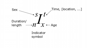
We distinguish between ultimate age ω (Greek omega) for indicating the ultimate age and the last (open-ended) age $z$ (Latin symbol z) of the population to be projected. We also distinguish between events in a period-cohort format or cohort events for short, denoted with a left upper superscript of c, period-age events (lacking the left upper subscript).

Table 1: Symbols of demographic indicators

Symbol	Description
$x$	Exact age; age at the beginning of an age group
$n$	Width of an age group
$\omega$	Last age of life table (begin of last, open-ended age group)
$z$	Last age of population (begin of last, open-ended age group)
$t$	Time (point of time, date)
$t,t + n$	Time period from t to t+n
${}_nP_x^t$	Population at time t in age group x to x+n
${}_nB_x^{t,t + n}$	Births by age of mother in age group x to x+n during period [t, t+n]
${}_nBp_x^{t,t + n}$	Births by age of mother in age group x to x+n during period [t, t+n] that are present at the beginning of the interval
${}_nBm_x^{t,t + n}$	Births by age of migrant mothers (in or out) in age group x to x+n during period [t, t+n]
${B^{t,t + n}}$	Total births during period [t, t+n]
${}_nM_x^{t,t + n}$	Migration in age group x to x+n during period [t, t+n], [P-A]
${}_n^cM_x^{t,t + n}$	Cohort migration (period-cohort format [P-C]).
${}_n^cD_x^{t,t + n}$	Cohort deaths (period-cohort format [P-C]).
${}_n^uD_x^{t,t + n}$	Deaths occurring in an upper Lexis triangle¹²
${}_n^lD_x^{t,t + n}$	Deaths occurring in a lower Lexis triangle
${}_n^cDm_x^{t,t + n}$	Cohort deaths to migrants, or deaths to those migrants that were aged x to x+n at time t at the beginning of the period [t, t+n], (period-cohort format [P-C]).
${}_nD_x^{t,t + n}$	Period deaths (period-age format), deaths to those that were aged x to x+n during the period [t, t+n]
${l_x}$	Life table survivor at exact age x
${}_n{d_x}$	Life table deaths between age x and x+n (deaths by age)
${}_n{L_x}$	Life table population in age group x to x+n (person-years lived in age group x to x+n, or stationary population)
${}_nS_x^{t,t + n}$	Life table survivor ratio; ratio of population in age group x to x+n to population x+n to x+2n.
${}_nW_x^{t,t + n}$	Withdrawal ratio, complement of the survivor ratio (1-S); ratio of withdrawals to population present at the beginning of the interval.
${}^c{{\rm{f}}_x}$	Cohort separation factor
${}^c{y_x}$	Cohort separation ratio

6 Bibliography

Bohk, C. (2011). Ein probabilistisches Bevölkerungsprognosemodel. Springer VS, Wiesbaden. (A probabilistic population projection model)

Bretz, M. (2000). Methoden der Bevölkerungsvorausberechnung in: Müller U., Nauck B., Dieckmann A. “Handbuch der Demographie” Band 1, S. 643-681.

Hill, K. (1990). PROJ3S – A Computer Program for Population Projections: Diskettes and Reference Guide.

Human Fertility Database. Max Planck Institute for Demographic Research (Germany) and Vienna Institute of Demography (Austria). Available at www.humanfertility.org.(10.08.2012)

Pavia, J. M., F. Morillas and J. Lledo (2012). Introducing migratory flows in life table construction. Statistics and Operations Research Transactions, Vol. 36, No.1, pp. 103-114.

Pollard, A. H., Farhat Yusuf, and G.N Pollard (1990). Demographic Techniques. Third edition. Pergamon Press

Preston, S., N. Keyfitz, and R. Schoen. 1972. Causes of Death: Life Tables for National Populations. New York: Seminar Press.

Preston, S. H., P. Heuveline, and M. Guillot (2001). Demography: Measuring and Modeling Population Processes, Blackwell.

Rowland, D.T. (2003). Demographic methods and concepts. Oxford University Press.

Swanson, D.A. and J.S. Siegel (2004) The Methods and Materials of Demography, Second Edition, Emerald Group Publishing.

UK (2012). Background and Methodology, 2010-based NPP Reference Volume, In National Population Projections, 2010-based reference volume: Series PP2.

UNPD (2015). Extended Model Life Tables (Version 1.3). United Nations Population Division, New York. https://esa.un.org/unpd/wpp/Download/Other/MLT/.

Wilmoth et al. (2007). Methods Protocol for the Human Mortality Database. Version 5. In Human Mortality Database. University of California, Berkeley (USA), and Max Planck Institute for Demographic Research (Germany). Available at www.mortality.org or www.humanmortality.de

See, for instance, the approach used by the US Census Bureau that is using exposure-occurrence rates centered around mid-period and explicitly including half-year intervals. Bokh (2011) used a similar approach. Other authors (Hinde 1999. Statistics UK, DESTATIS 2011, Breetz, 2000.) formulate the mathematics of the projection method in terms of true probabilities, which may be confusing. It seems that there is no authoritative, consistent and comprehensive mathematical description of the cohort-component available.↩
This option is named “mid-point adjustment” in Hill (1990).↩
Note that the formula for calculating births in an open population in Preston et al. (2001), p. 128 is not correct. By adding half the net-migration to the population at the beginning and half to the (projected) population at the end of the interval, net migration is inadvertently added a second time – it is already part of the (projected) population at the end of the interval.↩
The symbol p denoting population present at beginning↩
The symbol m denoting migrants.↩
Some implementations of the cohort-component model ignore the contribution of migrants to the first age group altogether.↩
This approach is used by Hill (1990), but with the multiplicative variant of implementing fractional risk (see Annex III)↩
Pollard did not give an empirical justification for his proposal.↩
The symbol p denotes population at the beginning of the interval.↩
Some implementations of the cohort-component model ignore the contribution of migrants to the first age group altogether.↩
Pollard did not give an empirical justification for his proposal.↩
Lower and upper triangles are sometimes denoted with the symbols α and δ, respectively (Keyfitz, 1968; Siegel, Swanson, 2004, p. 308)↩

Cohort-component algebra

1 Introduction

2 Synopsis: Cohort-component projection for open populations

2.1 Forward projection

2.1.1 Births

2.1.2 Survival of births

2.1.3 Projecting closed age groups

2.1.4 Projecting the last, open-ended age group, standard age format

2.1.5 Projecting the last, open-ended age group, extended age format

2.2 Calculation of deaths

2.2.1 Births

2.2.2 Closed age groups

2.2.3 Last, open-ended age group

2.3 Transformation of cohort deaths into death by age

2.3.1 First age group

2.3.2 Other closed age groups

2.3.3 Last, open-ended age group

2.3.4 Approximation I

2.3.5 Approximation II

3 Closed population

3.1 Forward Projection

3.1.1 Births

3.1.2 Survival of births

3.1.3 Projecting closed age groups

3.1.4 Projecting the last, open-ended age group, standard age format

3.1.5 Projecting the last, open-ended age group, extended age format

3.2 Calculation of cohort deaths

3.2.1 Births

3.2.2 Closed age groups

3.2.3 Last, open-ended age group, standard age format

3.2.4 Last, open-ended age group, extended age format

4 Open population

4.1 Forward projection, split migration option

4.1.1 Births

4.1.2 Survival of Births

4.1.3 Projecting closed age groups

4.1.4 Projecting the last, open-ended age group, standard age format

4.1.5 Projecting the last, open-ended age group, extended age format

4.2 Calculation of cohort deaths

4.2.1 Births

4.2.2 Closed age groups

4.2.3 Last, open-ended age group

4.3 Forward projection, mid-period migration option

4.3.1 Births

4.3.2 Survival of Births

4.3.3 Projecting closed age groups

4.3.4 Projecting the last, open-ended age group

4.4 Calculation of cohort deaths

4.4.1 Births

4.4.2 Closed age groups

4.4.3 Last, open-ended age group

5 Indicators and symbols

6 Bibliography